Leveraging explanation quality for model selection

In this notebook we are going to explore how, using teex, we can improve our model selection procedures (following Jia et al. (2021)).

0. How to do it?

Intuitively, a model that has a good predictive performance and makes decisions based on reasonable evidence is better than one that achieves the same level of accuracy but makes decisions based on circumstantial evidence. So, given an explanation model, we can investigate which evidence a model is basing its decisions on: a quality explanations will be of quality if it’s based on reasonable evidence and of low quality otherwise. Then, given two models with similar predictive performance, we should leverage whether or not it is basing its decisions based on good or bad evidence. Given this intuition, we define a model scoring mechanism:

\[score(f) = \alpha \cdot \text{score}_{acc}(f) + (1 - \alpha)\cdot \text{score}_{\text{explanation}}(f)\]

where \(\alpha\) \(\in[0, 1]\) is a hyperparameter, \(f\) is the model being assessed and \(\text{score}_{acc}(f)\) and \(\text{score}_{\text{explanation}}(f)\) are accuracy and explanation scores, respectively. All models \(f_1, ..., f_n\) will be assigned a score and we will choose based on it. teex will help us compute \(\text{score}_{\text{explanation}}(f)\).

import matplotlib.pyplot as plt
import numpy as np

from teex.saliencyMap.data import OxfordIIIT
from teex.saliencyMap.eval import saliency_map_scores

1. Getting the data

We are going to work with a subset of the Oxford-IIIT Pet dataset, included in teex. It contains roughly 7000 images from 37 categories.

from teex.saliencyMap.data import OxfordIIIT

data = OxfordIIIT()

We have the following classes available

data.classMap

{0: 'cat_Abyssinian',
 1: 'dog_american_bulldog',
 2: 'dog_american_pit_bull_terrier',
 3: 'dog_basset_hound',
 4: 'dog_beagle',
 5: 'cat_Bengal',
 6: 'cat_Birman',
 7: 'cat_Bombay',
 8: 'dog_boxer',
 9: 'cat_British_Shorthair',
 10: 'dog_chihuahua',
 11: 'cat_Egyptian_Mau',
 12: 'dog_english_cocker_spaniel',
 13: 'dog_english_setter',
 14: 'dog_german_shorthaired',
 15: 'dog_great_pyrenees',
 16: 'dog_havanese',
 17: 'dog_japanese_chin',
 18: 'dog_keeshond',
 19: 'dog_leonberger',
 20: 'cat_Maine_Coon',
 21: 'dog_miniature_pinscher',
 22: 'dog_newfoundland',
 23: 'cat_Persian',
 24: 'dog_pomeranian',
 25: 'dog_pug',
 26: 'cat_Ragdoll',
 27: 'cat_Russian_Blue',
 28: 'dog_saint_bernard',
 29: 'dog_samoyed',
 30: 'dog_scottish_terrier',
 31: 'dog_shiba_inu',
 32: 'cat_Siamese',
 33: 'cat_Sphynx',
 34: 'dog_staffordshire_bull_terrier',
 35: 'dog_wheaten_terrier',
 36: 'dog_yorkshire_terrier'}

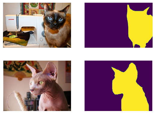
We are going to work in a binary setting, so let us choose two cat targets.

imSi, labSi, exSi = data.get_class_observations(32) # Siamese cats
imSp, labSp, exSp = data.get_class_observations(33) # Sphynx cats

f, axarr = plt.subplots(2,2)
axarr[0,0].imshow(np.array(imSi[5]))
axarr[0,0].axis("off")
axarr[0,1].imshow(np.array(exSi[5]))
axarr[0,1].axis("off")
axarr[1,0].imshow(np.array(imSp[4]))
axarr[1,0].axis("off")
axarr[1,1].imshow(np.array(exSp[4]))
axarr[1,1].axis("off")

(-0.5, 499.5, 374.5, -0.5)

2. Declaring a classifier

# WIP...